3. Thermo-compositional convection

In this demo, we will mimic a dense dyke injected into an ice shell, its collapse and entrainment by thermal convection.

Thermo-compositional convection in an ice shell.

Download

Here you can download the complete parameter file , the modified material properties fileand the matplotlib scriptfor the animation.

Material properties file modification

We add the dependence of ice density on the composition, enhancing the density where the dyke material is present.

\[\rho(T, C) = \rho_i(T)\cdot (C_{\rm ice} + 1.004\cdot C_{\rm salt})\]

def rho(Temp, composition, xm):
        # .
        # .
        # .
        return ((1.0-xm)*rho_s*mm/VV + xm*rho_m)*(composition[0] + 1.004*composition[1])

Parameter file modification

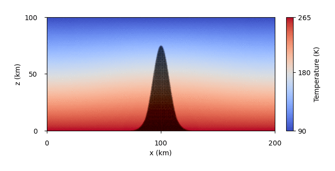
In the parameter file, we modify the interface() function as a gaussian peak in the middle of the ice shell to represent the dyke. Afterwards, in the first position of materials, we enter the whole domain (the ice), and in the second position the dyke material defined as the material below the interface.

def interface(x):
    return 75e3*exp(-(x - 100e3)**2/1e8)

# --- Leave empty for a single material ---
materials = [["rectangle",  0, length, 0, height], ["interface",  "below"]]

To resolve the dyke well, we refine the lower half of the domain (same as in the original example) and the region that contains the dyke.

refinement = [0, length, 0, height/2, 80e3, 120e3, height/2 + 1e3, 80e3]