3. Thermal convection with phase transition

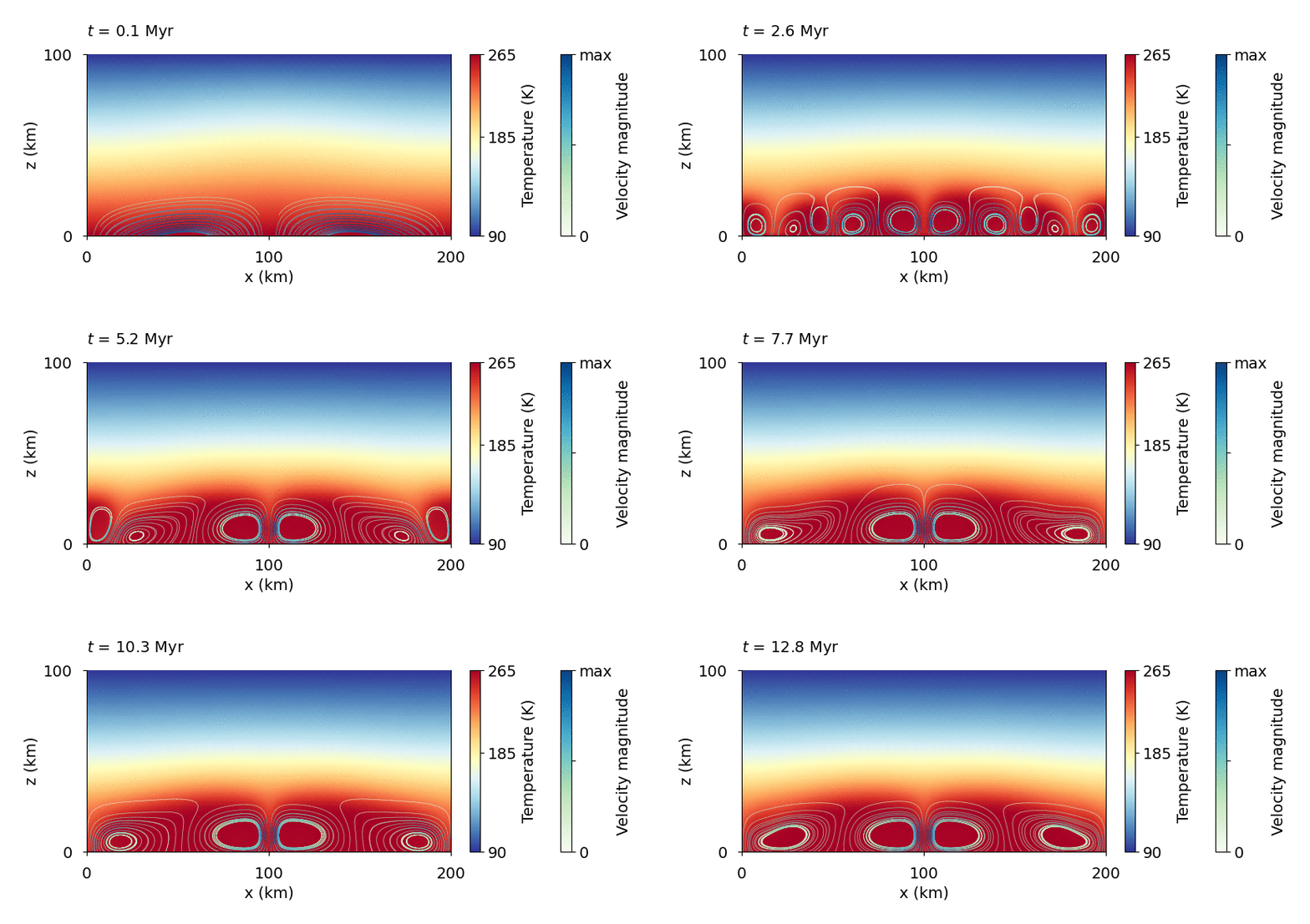
_images/demo3.gif — Thermal convection in an ice shell with a phase transition at the bottom boundary. Note the difference in temperature structure compared to the case with closed boundary . The contours represent the streamlines and their color scales the maximum speed at given time step.

Download

Here you can download the bash script, the parameter fileand the matplotlib scriptfor the heat flux evolution. Detailed explanation is given below.

Note

Copy the bash script, parameter file, and plotting script from /demos/demo3/ into the main directory.

Parameter file modification

First, we redefine the directory name:

# --- Name of the directory with results ---
name = "demo3_convection_phase1e15"

Then, we make the output more frequent.

output_frequency = ["time", 50*kyr]

Compared to the thermal convection in the previous section, we need the bottom boundary to deform, therefre we prescribe the free surface boundary condition

# Boundary conditions for velocity (free_slip, no_slip, free surface, velocity, velocity_x, velocity_y)
BC_Stokes_problem = [["free_slip"],      # top boundary       (1)
                    ["pressure"],        # bottom boundary    (2)
                    ["free_slip"],       # left boundary      (3)
                    ["free_slip"]]       # right boundary     (4)

In order to shape the boundary by the phase transition (melting and crystallization), we turn the phase transition on. The DAL_factor determines the “strength” of the Deguen-Alboussière-Labrosse effect. The value 10 mW/m ^-3 should result in significant ocean-shell exchange.

# --- Phase transition at the bottom boundary ----
phase_transition = True

# --- Strength of the phase transition at the ice-water boundary ---
DAL_factor  = 1e-2 # W/m3

Finally, we prescribe the temperature-dependent viscosity one order of magnitude hugher than in the first example

# --- VISCOSITY ---
viscosity_type = "temp-dep"
.
.
.
# --- Parameters for constant / temperature-dependent viscosity ---
eta_0 = 1e15

Visualization of streamlines

First, in plot_demo3.py, we define points (50 points evenly distributed along the domain length, placed 2 km above the bottom boundary) whose trajectories will be evaluated.

# --- Starting points for streamlines computation ---
length = 200e3 # Length of the domain
num_points = 50
points = []
for i in range(1, num_points):
    if (i != int(num_points/2.0)):
        points.append([length/num_points*i, 2e3])

Then, function compute_streamlines() preforms numerical integration of trajectory of the points defined above and visualizes the streamlines.